Data visualization is one of the stages of analysis, but usually one of the final steps – on its basis we can assess the condition of our business, draw conclusions or propose recommendations. However, before we reach this stage, first we need to prepare and model the data. The old analytical saying states that each analyst spends 80% of their time on preparing the data, and 20% on the analysis. For this reason, all leading Business Intelligence tools offer some form of the ETL (Extract, Transform, Load). For Tableau it’s Prep, and for Power BI – Power Query. The market of ETL tools is quite wide, and it offers a lot of basic and advanced programs. However, for the majority of basic business applications, the ETL add-ons would be sufficient. This way we can easily connect to the source, model the data and load the prepared model to Power BI (or Tableau) and carry out proper analysis. How to start modelling data with the help of Power Query?
Connecting and loading data using Power Query
The first step is to connect the data. Power Query can be initiated from the level of Power BI – by clicking the “Transform data” field. The data can be connected by selecting “Get data”. There are many connections available, from the basic cvs or xls to the online Azure or Salesforce.
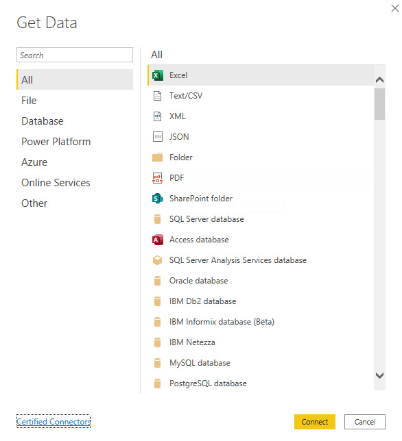
For training purposes, we will connect to the data with the results of football matches. After selecting the option File -> Text/CSV, we are able to view our data:
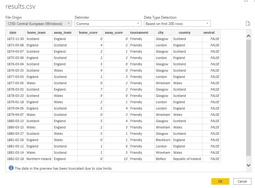
We click OK to load our data and start modelling and transforming the data. The main window of Power Query is similar to other Microsoft applications. On the top there is a ribbon with the available options, in the middle the main view of the table and on the left, there is a list search results (data connections), while on the right we have a list of actions performed during modelling. It’s a very practical functionality which enables us to see the transformations which are performed on our data and int what order. In addition, once we define the steps, there is no need to define them again – when creating the transformation, we have to do that only one time. The list and steps can be edited, which simplifies adding modifications at a later stage.

Cleaning, modelling and transforming data in Power Query
Once the data is loaded, we can start the tedious process of data cleaning to prepare it for analysis. When the data is connected, Power Query will automatically create three steps:
1. Source – connecting the data
2. Promoted Headers – treating the first row of the table as headers
3. Changed Type – determining the type of data
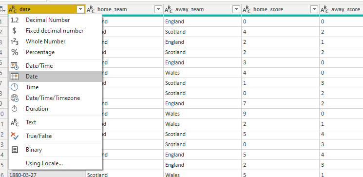
The third point is performed automatically based on the data sample; therefore, it is not always right. In our case, the model has wrongly identified the date. Text was chosen instead of Date. We can easily change it by clicking the type of data in the header:
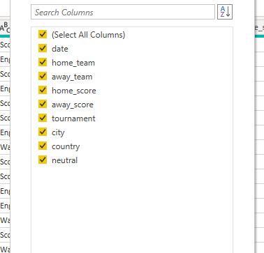
The next stage is to select the relevant columns. A good practice is to leave only the ones which are needed for further analysis. This way our model will not only transparent, but it will also take less space and be quicker.
Once columns are selected, we move on to rows. If our data contains errors, empty values or duplicates – we can eliminate them at this stage by choosing appropriate options. In our case, we are going to delete the rows with incorrect data.
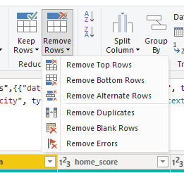
It’s worthwhile to pay attention to the way, in which Power Query executes our commands. By selecting appropriate options from the graphic interface – the commands on the ribbon – Power Query creates formulas in the M language. We can view them in the formula tab similarly to Excel:

Other options in the ribbon allow us to split or format the columns and to extract the required values. Let’s assume that we want to extract the year from the data. We can do that using the split option:
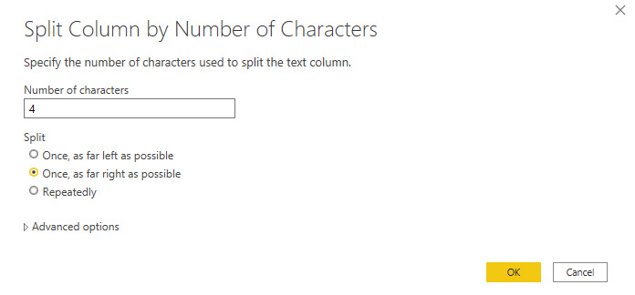

Or the Extract command:
The advantage of the second option is that the new column replaces the old one. In the case of the Split command, we receive two columns, which means that we need to add another step to delete the first column. It’s often the case when modelling the data in Power Query – the desired effect can be achieved in a number of ways. We should always aim for the easiest one to ensure the effectiveness of our model.
Data modelling – expanding the data model by adding new elements
With the help of Power Query, we can add new calculation columns to our data table – by using the Add Column ribbon. We can choose from several options, and the formulas can be entered in the editor available after selecting the Custom Column option. In the analyzed case, we are going to add a column with the number of goals in the match, which consists of the sum of goals scored by the home team and the away team:
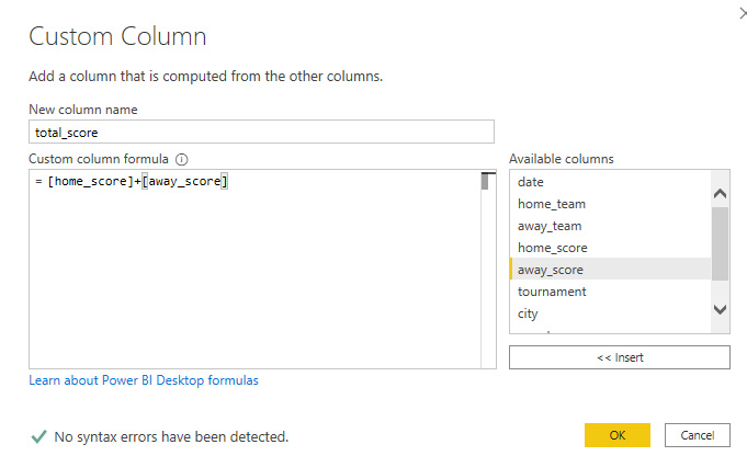
The formulas are defined in the aforementioned M language. It’s pretty intuitive in basic applications, but it requires some experience for more advanced ones. Therefore, the Conditional Column editor is extremely helpful – it allows us to arrange the rules according to function, as it is in Excel. Let’s assume that we want to add a column which shows who won the match: the home team, the away team or a draw. The function defined in the editor looks as follows:
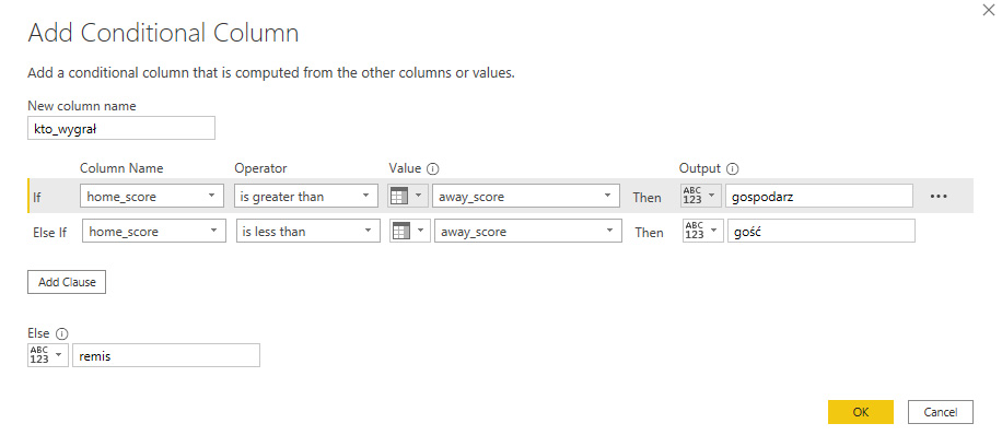
Whereas the function in the M language generated by the editor looks as shown below. If you are an experienced user of logical functions, for example in Excel, you will easily read the syntax of the function.

Our table can be further expanded by adding other columns to it. Search results can be combined either by:
1. Append – we add tables in the same layout one under the other
2. Merge – we add the data from the other table to the main table, which is searched by the defined key.
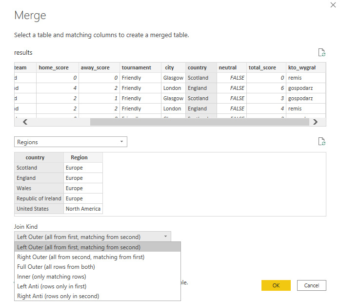
The merge option works similarly as in the case of combining tables with the join function. When selecting the Merge option, you need to indicate the table that you want to add, the fields, in which the items will be search and the type of joint (left, right, full, inner). In the analyzed example, we want to add the information about the region where the matches took place to the main table. We search the “country” field using the Left Outer join.
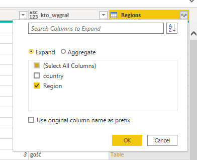
Once the tables are joined, all we need to do is to select the fields we want to display from the connected table in our base table:
Next, we can load the data to the model to start the data analysis and visualization process in Power BI.
Power Query is a very practical and user-friendly ETL
Power Query is an excellent ETL tool. The interface is user-friendly, and it’s intuitive for users who have worked with Microsoft products. The graphic editor allows us to model the data without knowing the M language or any SQL language. Therefore, we can easily perform basic transformations. A great option is the window with the applied steps during the data modelling stage, which allows us to see what’s happening with the data at each stage. This way we can easily track down the path and edit it when business needs change. The data processed in Power Query is immediately available for visualization in the integrated Power BI, which all together gives us a coherent self-service BI package.
Data modelling – Tableau Prep or Power Query?
The question is similar to whether to choose Power BI or Tableau. The answer isn’t straightforward as a lot depends on the user’s preferences. In terms of functionality, the tools are remarkably similar – both are ETL tools that support data modelling and transforming. Both prepare the data for further analysis and visualization in Power BI or Tableau. The advantage of Tableau Prep is that it generates ready extracts to be analyzed in Tableau. We don’t need to export the data to cvs files. Power Query – as it is integrated with Power BI, doesn’t require to run a separate application (as Prep), which also makes our work easier. Power Query interface will also be easier to learn for beginners, as it’s similar to other applications such as Excel. On the other hand, Tableau Prep is excellent at visualizing data flows, allowing us to see how the data is modelled. Therefore, it’s hard to clearly indicate which of them is definitely better – they both are good ETL tools.
Mateusz Karmalski,
Tableau Author
